Six months ago I blogged a model for optimal stop spacing on an urban transit route. These models exist in the published literature, but they assume that the speed benefit of stop consolidation reduces operating costs, which requires introducing new variables for the value of time. My model assumes the higher speed of stop consolidation is plugged into higher frequency, which means only five variables are needed, and only two of them vary substantially between different cities and their networks. The formula is a square root.

In this post, I’m going to extend this formula to optimizing route spacing on a grid.

I’m using mode-neutral language like “vehicle,” but this is really just about buses, because to a good approximation, urban rail networks are never grids. I’m sorry, Mexico City, I know your Metro network does its best to pretend you have an isotropic city, but your three core radial lines are just far busier than the tangential ones.

Optimal stop spacing: a recap

My previous post uses words rather than symbolic language, since there are only five relevant parameters. Here I’m going to use symbols for the variables to make the calculation even somewhat tractable. All units I’m using are base SI units, so speed is expressed in meters per second rather than kilometers per hour, but the dimensional analysis works out so that it’s not necessary to pick units in advance.

• s: stop spacing
• v: walk speed
• p: stop penalty
• d: average distance traveled
• w: walk/wait penalty, expressed as a ratio of perceived walk or wait time to in-vehicle time
• λ: average distance between successive vehicles, or in other words headway in units of distance, not time

The variables v and p are fairly consistent from place to place. The variable w is as well, but may well differ by circumstance, e.g. people with luggage may have a higher walk penalty and a lower wait penalty, and people who are more familiar with the system usually have lower w. The parameter λ is a function of how much service runs on the line, as we will see when we expand to cover route spacing.

A key assumption in this model is that d does not change based on the network. This is a simplification: if s is too low then it will drag down d with it, as people who are discouraged by the slow in-vehicle speed avoid long trips or choose other modes of travel, whereas if s is too high then it will drag d up, as people who have to walk too long to the stop may just walk all the way to their destination if it’s nearby. In Carlos Daganzo’s textbook this situation is resolved by replacing an empirically determined d with the size of the city, assuming travel is isotropic, but the effect is essentially the same as just setting d to be half the length of a square city.

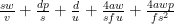
The formula for perceived travel time is

if travel along the line is isotropic, or

if one end of the travel (e.g. the residential end) is isotropic and the other is at a fixed node (e.g. a subway transfer). In either case, in-vehicle time excluding stops is omitted, as it is constant.

The minimum travel time occurs at

if travel is isotropic and

if there is a distinguished node at one end of the trip.

Observe that there is negative interaction between stop consolidation and other aspects of bus modernization. First, higher frequency, as expressed in concentrating service on strong routes, reduces the value of λ and therefore slightly reduces the optimal stop spacing. Second, the model assumes the same penalty w for walking and waiting, but sometimes these two activities have distinct penalties, and then the walk penalty is responsible for the occurrence of w in the denominator in the formula whereas the wait penalty supplies the appearance of w in the numerator. Improving bus stop facilities reduces the wait penalty, pushing the optimal s farther down, even though at the same time it’s cheaper to improve bus stops if there are fewer of them.

The empirically determined values of the five variables in the formula are as follows:

• v is 1.45 m/s in Forde-Daniel, 1.3-1.4 m/s in Bohannon, and 1.38 in TRB Part 4, PDF-p. 16; I take v = 4/3
• p is 25 seconds based on examining the differences in schedules between local and limited buses in New York and Vancouver
• d is 3,360 meters per unlinked trip per the NTD
• w is around 2 for waiting in Fan-Guthrie-Levinson, 2 in general for buses in Teulings-Ossokina-de Groot, PDF-p. 25, 1.75 in the New York MTA’s internal model, 2.25 in the MBTA’s (as mentioned in one of Reinhard Clever’s papers), and a range of 2-3 in Lago-Mayworm-McEnroe; I take w = 2
• λ is single-lane network length (that is, twice the route-length, modulo one-way loops) divided by fleet size in actual use, which is 1,830 meters in Brooklyn today and 1,160 based on what Eric Goldwyn and I recommend

This leads to optimal stop spacing equal to

if travel is isotropic and

if there is a distinguished node. The numbers are slightly lower than in my older post since I’m using a slightly lower walk speed, 1.33 m/s rather than 1.5.

Optimal route spacing: stops at intersection points

Studying route spacing has to incorporate stop spacing for a simple reason: there should be a stop at every intersection between routes, and therefore the route spacing should be an integer multiple of the stop spacing. There are three modifications required to the above formula, of which the first is easy, the second requires defining more parameters but is mathematically still easy, and the third is very hard:

1. Passengers need to walk not just along the route to their stop but also from their origin to the route, which increases walk time
2. The value of λ may change, since fewer routes imply more vehicles per route and thus denser vehicle spacing, and in particular wait time depends not just on how many stops are on the way but also on the speed net of stops
3. Increasing the route and stop spacing in tandem reduces the number of stops involved in waiting for the bus (this is λ again) twice, that is quadratically

The first modification means that instead of traveling an average distance of s/4 to the stop at each end, assuming isotropy, people have to travel a distance of s/4 along the route and also s/4 to the route itself. In the travel time formula, we replace sw/2v with just sw/v with isotropic travel.

To deal with the second modification, we define the following variables, in addition to the ones from the section above on stop spacing:

• f: fleet size in independent vehicles in actual revenue operation (buses or trains, not train cars)
• a: area of the network to be covered by the grid, e.g. a city, metro area, or borough
• u: speed assuming there are no stops along the route

If the area is a, then we can approximate it as a square of side , which has north-south and east-west routes, each of length , and thus the total two-way network length is 2a/s. Since the value of λ is the one-way length divided by fleet size, we write

Moreover, people wait an additional λw/2u; in the previous section this wait existed as well but was ignored in the formula as it did not depend on s, but here it does, and thus we need to add this wait factor.

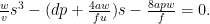
We deal with the third modification by replacing λ with 4a/sf in the formula for wait time. If people travel isotropically and do not transfer, the travel time formula is now

The summand d/u is constant but is included for completeness here, in analogy with the no-longer-constant summand 2aw/sfu.

But it’s the last summand that gives the most problems: it turns the optimization problem from extracting a square root to solving a cubic. This is technically possible, but the formula is opaque and does not really help showcase how the parameters affect the final outcome. We need to solve for s:

We can plug in the above values of w, v, d, and p, as well as the following values of the new variables, and use any cubic solver:

• f = 612 buses in Brooklyn, excluding vehicles in turnaround, non-revenue service, etc. (it’s actually slightly lower today, around 600, but our network is a bit more efficient with depot moves)
• a = 180,000,000 m^2 for Brooklyn
• u = 5.3 m/s net of stops, assuming our other proposals, such as bus lanes, are implemented

The cubic formula turns into

for which the positive solution is s = 528 meters.

We can complicate this formula in two ways.

First, we can let go of the assumption of isotropy. If there is a distinguished node at one end, then walk time is halved, as in the formula for stop spacing on a given route. The overall travel time is equal to

and this is optimized when

Plugging the usual values of the parameters, we get

for which the positive solution is s = 719 meters. The ratio between the results with isotropy and a distinguished node is 1.36, close to the square root of 2 that we get in the formula for stop spacing on a predetermined route; the reason is that in the cubic formula the linear term is much larger than the constant term near the root, so the effect of changing the cubic term is much closer to the square root than to the cube root.

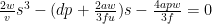
The second complication is introducing transfers. Transfers do not change the walk time – the walking time between platforms or curbside waiting areas is small and constant – but introduce additional wait time, which means we need to double both terms that include waits. But if we have transfers we need to restore the assumption of isotropic travel, since for the most part the distinguished nodes for Brooklyn buses involve subway transfers.

In that case, the travel time formula is

which is minimized at the positive root of the cubic

We need to figure out the value of d, which is difficult in this case – the New York bus network discourages bus-to-bus transfers through low frequency and poor bus stop amenities. That the formulas I’m using do not allow for how the shape of the network influences d is a real drawback here. But if we let d be the usual 3,360 meters that it is for unlinked trips, and plug the usual values of the other parameters, we get,

to which the solution is s = 683 meters.

Optimal route spacing: the general case

The above section makes a critical assumption about route spacing and stop spacing: they must be equal, making every stop a transfer. However, this assumption is not strictly necessary. Indeed, if we assume isotropy, and let the route spacing be 860 meters, then it’s better for passengers to double the density of stops to one every 430 meters just from looking at the formula for stop spacing.

In this section, we look at the optimal formulas assuming route spacing is twice or thrice the stop spacing. Then in the next section we will compare everything together.

We keep all the variable names from before, and set s to be the stop spacing, not the route spacing. Instead, we will find formulas for route spacing equal to 2s and 3s and compare their optima with that for the special case in which stop and route spacing are equal.

We need to modify the formula in the previous section in two ways. First, walk time is, in the isotropic case, half the stop spacing plus half the route spacing. And second, the dependence of λ on the shape of the network comes from route spacing rather than stop spacing. If route spacing is 2s, the formula for travel time is

and its minimum is at the positive solution to

We retain the New York- and Brooklyn-oriented variables from the above sections and obtain

The solution is s = 352 meters, i.e. routes are to be spaced 704 meters apart, with one intermediate station on each route between each pair of successive crossing routes.

If we have three interstation segments between two successive routes, then we need to solve the cubic

or

to which the solution is s = 276 meters.

In the above section we also looked at two potential complications: introducing transfers, and introducing non-isotropy. Non-isotropy, expressed as an isotropic origin and a distinguished destination, halves the cubic term; transfers double the wait times and thus double the constant term and the larger of the two summands adding up to the linear term.

If the route spacing is exactly twice the stop spacing, then the non-isotropic formula is

or, using the same parameters as always,

The solution is s = 420 meters, with routes spaced 840 meters apart.

The isotropic cubic with transfers is

and with the usual parameters, again sticking with d = 3,360 even though in practice it is likely to be higher, this is

and then the root is s = 442 meters, with routes spaced 884 meters apart.

We conclude this section with the same formulas assuming the route spacing is not 2s but 3s. The non-isotropic, one-seat ride formula is

or with the usual parameters

of which the positive root is s = 374 meters, with routes spaced 1,123 meters apart,

The transfer-based isotropic formula is,

or

The positive root is s = 340 meters, with routes spaced 1,021 meters apart.

What’s the best route spacing?

We have optimums based on assumptions about the interaction between stop and route spacing, but so far we have not compared these assumptions with each other. In this section, we do. For each scenario – isotropic, transfer-free travel; a distinguished node along transfer-free travel; and isotropic travel with a transfer – we look at the optimal values of route spacing equal to one, two, or three times the stop spacing.

In the table below, the walk and wait times are without penalty; but the penalty is applied to them when summed with in-vehicle time.

Scenario	Component	Route spacing = s	Route spacing = 2s	Route spacing = 3s
Isotropy; 1-seat ride	Optimal s	528	352	276
	Walk time	396	396	414
	Wait time	262.954	216.997	198.394
	In-vehicle time	793.053	872.599	938.31
	Total time	2110.962	2098.593	2163.097
Distinguished node; 1-seat ride	Optimal s	719	420	374
	Walk time	269.625	236.25	280.5
	Wait time	182.811	173.812	133.965
	In-vehicle time	750.791	833.962	858.561
	Total time	1655.663	1654.086	1687.49
Isotropy; 2-seat ride	Optimal s	683	442	340
	Walk time	512.25	497.25	510
	Wait time	388.05	326.378	302.432
	In-vehicle time	756.949	824.008	881.021
	Total time	2557.549	2471.263	2505.885

 

The table implies that in all scenarios it’s optimal to have two interstations between parallel routes, though if there’s a distinguished node the difference with having just one interstation between parallel routes is very small. The three-interstation option is never optimal, but is also never far from the optimum, only half a minute to a minute worse.

But please interpret the table with caution, especially the two-seat ride section. The total time for a 3.36-kilometer trip without applying the walk or wait penalty is about 28 minutes regardless of whether the route to stop spacing ratio is 1, 2, or 3. This is still faster than walking, but not by much, and riders may well be so discouraged as to walk the entire way. If the trip is much shorter than 3.36 kilometers or the rider’s particular disutility of walking is much lower than 2 then transit will not be competitive with walking. In turn, a network set up with the stop spacing implied by the above formulas will only get transfer trips if they’re much longer, which should raise the optimal interstation somewhat. If d = 6,000 then in the transfer scenario the optimum if stop and route spacing are equal is 711 meters and that if route spacing is twice as high as stop spacing is 470 meters, and the latter option is noticeable faster.

How does our bus redesign compare with the theory?

We drew our redesigned map with full knowledge of how to optimize stop spacing on a single route, but we didn’t look at route spacing optimization. Of course, the assumption of regular route spacing is less realistic than that of regular stop spacing, as some areas have higher demand, or more distinguished arterials. But we can still discuss the average route spacing in our plan, by comparing our proposed route-length with Brooklyn’s land area.

With a 356-kilometer network in a borough of 180 km^2, effective route spacing is 1,010 meters. This is a little longer than I expected; in Southern Brooklyn the north-south and east-west routes we propose are spaced around 800-850 meters apart, and in Bed-Stuy the east-west routes tighten to 600 meters as they’re all radial toward Downtown Brooklyn and quite busy. The reason the answer is 1,010 meters is that there are margins of the borough with no service (like Floyd Bennett Field) or grid interruptions due to parks (such as Prospect Park) or already-good subway service (South Brooklyn).

The stop spacing we use is 480 meters, excluding nonstop freeway segments in the Brooklyn-Battery Tunnel and toward JFK. In the Southern Brooklyn grid, we’re pretty close to a regular spacing of two interstations between parallel routes. In the Bed-Stuy grid, the north-south routes have a stop per crossing route since the east-west routes are so densely placed, and the east-west routes have one, two, or three interstations between crossing routes, but the average is two.

To the extent the optimization formulas tell us anything, it’s that we should consider adding a few more routes. Target additions include another north-south Bed-Stuy route, an east-west route in South Brooklyn restoring the discontinued B71, and a north-south route through Southern Brooklyn on 16th Avenue. Altogether this would add around 20 km to our network. Beyond that, additional routes would duplicate subway routes, which my analysis above excludes even when they form a coherent grid with the buses.

Rules of thumb for your city

If your city has streets that form a coherent grid, then you can design a bus grid without too many constraints. By constraints I mean street networks that interrupt the grid so often so as to force you to use particular streets at particular spacing, for example the Bronx or Queens. Constraints in a way make planning easier, by reducing the search space; I contend Brooklyn is the hardest of the four main boroughs to redesign precisely because it has the fewest constraints in its grids and yet its grid is just interrupted enough that it cannot be treated as tabula rasa.

In general, you probably want buses spaced around 800 meters to a kilometer apart. While the value of d will differ between cities, the optimum route spacing isn’t that sensitive to it. If d rises to as high as 10,000, the optimal s in the scenario with transfers is 753 meters if route spacing equals stop spacing and 511 meters if it equals twice stop spacing, compared with 683 and 442 meters respectively with d = 3,360; the one-interstation-per-parallel-route scenario becomes better than the two-interstation scenario, but the difference is half a minute, compared with a minute and a half in favor of two interstations with d = 3,360.

In practice I don’t know of any city whose grid is so unconstrained and so isotropic that you can seriously debate 700, 800, 900, 1,000, etc. meters between routes. At that resolution you’re always constrained by arterial spacing, which in American cities tends to be 800 because it’s half a mile and in Canada is irregular (de facto close to a mile) due to constant grid interruptions on intermediate would-be arterials in both Toronto and Vancouver. In this range of arterial spacing, you want exactly two interstations between parallel routes; if you want more or fewer then you should have a very good reason, such as a major destination such as a hospital located at an awkward offset.

Something that does matter very much is fleet size relative to the area served – the quantity a/f. If you aren’t running much service, then you need wider route spacing just to avoid reducing frequency to unusable levels. If instead of f = 612 we use f = 200, then the optimum with one interstation per parallel routes with the transfer scenario is s = 1087, with two it’s s = 676, with three it’s s = 508, and with four it’s s = 414, and among these three is best and even four is a few seconds faster than two. In that case route spacing of about a kilometer and a half, which may be a mile in American arterials, is fully justified.

Conversely, if buses are faster, that is if u is higher, then the optimal interstations fall in all cases. This is because the impact of u comes from its effect on wait times, so faster buses mean that it’s less important to reduce λ.

The effects of a/f and u relate again to the negative interactions between various components of bus reform. Running more service means it’s justifiable to have more closely-spaced routes, since pruning routes to increase frequency from 10 to 5 minutes is much less valuable than pruning them to increase frequency from 30 to 15 minutes. Likewise, running faster service means wait times fall, again reducing the need to prune routes.

If you’re tasked with designing bus routes, then make sure to use correct values for a, f, u, and d for your city, as they are likely to be very different from those of New York. The formulas are more intricate when optimizing route spacing and it’s useful to play with them until you get comfortable with them on an intuitive level, but ultimately they do give reasonable answers for how to design a bus network.