Optimization
This post may be of general interest to people looking at optimization as a concept; it’s something I wish I’d understood when I taught calculus for economics. The transportation context is network optimization – there is a contrast between the sort of continuous optimization of stop spacing and the discrete optimization of integrated timed transfers.
Minimum and maximum problems: short background
One of the most fundamental results students learn in first-semester calculus is that minimum and maximum points for a function occur when the derivative is zero – that is, when the graph of the function is flat. In the graph below, compare the three horizontal tangent lines in red with the two non-horizontal ones:
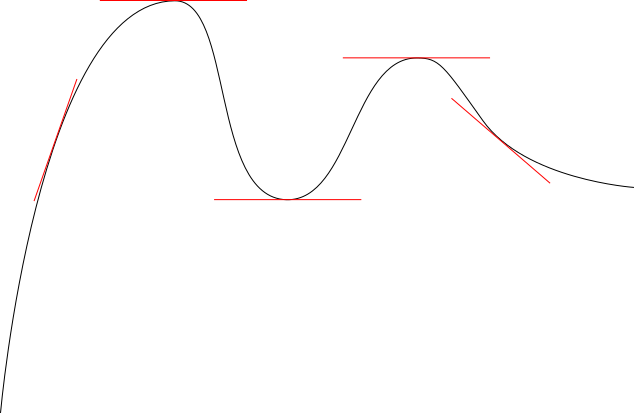
A nonzero derivative – that is, a tangent line slanting up or down – implies that the point is neither a local minimum nor a local maximum, because on one side of the point the value of the function is higher and on the other it is lower. Only when the derivative is zero and the tangent line is flat can we get a local extreme point.
Of course, a local extreme point does not have to be a global one. In the graph above, there are three local extreme points, two local maxima and one local minimum, but only the local maximum on the left is also a global maximum since it is higher than the local maximum on the right, and the local minimum is not a global minimum because the very left edge of the graph dips lower. In real-world optimization problems, the global optimum is one of the local ones, rather than an edge case like the global minimum of the above graph.
First-semester calculus classes love giving simplified min/max problems. This class of problems is really one of two or three serious calc 1 exercises; the other class is graphing a function, and the potential third is some integrals, at universities that teach the basics of integration in calc 1 (like Columbia and unlike UBC, which does so in calc 2). There’s a wealth of functions that are both interesting from a real-world perspective and doable by a first-semester calc student, for example maximizing the volume of some shape with prescribed surface area.
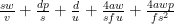
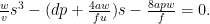
My formulas for stop spacing come from one of these functions. The overall travel time is a function of walking time, which increases as stops get farther apart, and in-vehicle time, which decreases as stops get farther apart. A certain stop spacing produces the minimum overall trip time; this is precisely the global minimum of the travel time function, which is ultimately of the form 
Continuous optimization
The fundamental fact of continuous optimization, one I wish I’d learned in time to teach it to students, is that at the optimum the derivative is zero, and therefore making a small mistake in the value of the optimum is not a big problem.
What does “mistake” mean in this context? It does not mean literally getting the computation wrong. There is no excuse for that. Rather, it means choosing a value that’s slightly suboptimal for ancillary reasons – perhaps small discontinuities in the shape of the network, perhaps political considerations.
Paul Krugman brings this concept up in the context of wages. The theory of efficiency wages asserts that firms often pay workers above the bare minimum required to get any workers at all, in order to get higher-quality workers and incentivize them to work harder. In this theory, the wage level is set to maximize employer productivity net of wages. At the employer’s optimum the derivative of profit is by definition zero, so a small change in wages has little impact to the employer. However, to the workers, any wage increase is good, as their objective function is literally their wage rather than profits. They may engage in industrial action to raise wages, or push for favorable regulations like a high minimum wage, and these will have a limited effect on profits.
In the context of transit, this has the obvious implication to wages – it’s fine to set them somewhat above market rate since the agency will get better workers this way. But there are additional implications to other continuous variables.
With stop spacing specifically, the street network isn’t perfectly continuous. There are more important and less important streets. Getting transit stops to align with major streets is important, even if it forces the stop spacing to be somewhat different from the optimum. The same is true of ensuring that whenever two transit lines intersect, there is a transfer between them. This is the reason my bus redesign for Brooklyn together with Eric Goldwyn involved drawing the map before optimizing route spacing – the difference between 400 and 600 meters between bus stops is not that important. For the same reason, my prescription for Chicago, and generally other American cities with half-mile grids of arterial roads, is a bus stop every 400 meters, to align with the grid distance while still hewing close to the optimum, which is about 500.
When I talked about stop consolidation with a planner at New York City Transit who worked on the Staten Island express bus redesign, the planner explained the philosophy to me: “get rid of every other stop.” In the context of redesigning a single route, this is an excellent idea as well: the process of adding and removing bus stops in New York is not easy, so minimizing the net change by deleting stops at regular intervals so as to space the remaining stops close to the optimum is a good idea.
The world of public transit is full of these tradeoffs with continuous variables. It’s not just wages and interstations. Fares are another continuous variable, involving particular tensions as different political factions have different objective functions, such as revenue, social rate of return, and social rate of return for the working class alone. Frequency is a continuous variable too in isolation. Top speed for a regional train is in effect a continuous variable. All of these have different optimization processes, and in all cases, it’s fine to slightly deviate from the strict optimum to fulfill a different goal.
Discrete optimization
Whereas continuous optimization deals with flat tangent lines, discrete optimization may deal with delicate situations in which small changes have catastrophic consequences. These include connections between different lines, clockface scheduling, and issues of integration between different services in general.
An example that I discussed in the early days of this blog, and again in a position paper I just wrote to some New Hampshire politicians, is the Lowell Line, connecting Boston with Lowell, a distance of 41 km. The line is quite straight, and were it electrified and maintained better, trains could run at 160 km/h between stops with few slowdowns. The current stop spacing is such that the one-way trip time would be just less than half an hour. The issue is that it matters a great deal whether the trip time is 25 or 27 minutes. A 25-minute trip allows a 5-minute turnaround, so that half-hourly service requires just two trainsets. A 27-minute trip with half-hourly service requires three trainsets, each spending 27 minutes carrying passengers and 18 minutes depreciating at the terminal.
A small deterioration in trip time can literally raise costs by 50%. It gets to the point that extending the line another 50 kilometers north to Manchester, New Hampshire improves operations, because the Lowell-Manchester trip time is around 27-28 minutes, so the extension can turn a low-efficiency 27-minute trip into a high-efficiency 55-minute trip, providing half-hourly service with four trainsets.
In theory, frequency is a continuous variable. However, in the range relevant to regional rail, it is discrete, in fractions of an hour. Passengers can memorize a half-hourly schedule: “the inbound train leaves my stop at :10 and :40.” They cannot and will not memorize a schedule with 32-minute frequency, and needing to constantly consult a trip planner will degrade their travel experience significantly. Not even smartphone apps can square this circle. It’s telling that the smartphone revolution of the last decade has not been accompanied with rapid increase in ridership on transit lines without clockface schedules, such as those of the United States – if anything, ridership has grown faster in the clockface world, such as Germany and Switzerland.
Transit networks involving timed connections are another case of discrete optimization in which all parts of the network must work together, and small changes can make the network fall apart. If a train is late by a few minutes and its passengers miss their connection, the short delay turns into a long one for them. As a result, conscientious schedule planners make sure to write timetables with some contingency time to recover from delays; in Switzerland this is 7%, so in practice, out of every 15 minutes, one minute is contingency, typically spent waiting at a major station.
But this gets even more delicate, because different aspects of the transit network impact how reliable the schedule is. If it’s a bus, it matters how much traffic there is on the line. Buses in traffic not reliable enough for tight connections, so optimizing the network means giving buses dedicated lanes wherever there may be traffic congestion. Even though it’s a form of optimization, and even though there’s a measure of difficulty coming from political opposition by drivers, it is necessary to overrule the opposition, unlike in continuous cases such as wages and fares.
Infrastructure planning for rail has the same issues of discrete optimization. It is necessary to design complex junctions to minimize the ability of one late train to delay other trains. This can take the form of flying junctions or reducing interlining; in Switzerland there are also examples of pocket tracks at flat junctions where trains can wait without delaying other trains behind them. Then, the decision of how much to upgrade track speed, and even how many intermediate stations to allow on a line, has to come from the schedule, in similar vein to the Lowell Line’s borderline trip time.
Continuous and discrete optimization
Many variables relevant to transit are in theory continuous, such as trip time, frequency, stop spacing, wages, and fares. However, some of these have discontinuities in practice. Stop spacing on a real-world city street network must respect the hierarchy of more and less important destinations. Frequency and trip times are discrete variables except at the highest intensity of service, perhaps every 7.5 minutes or better; 11-minute frequency is worse to the passenger who has to memorize a difficult schedule than either 10- or 12-minute frequency.
New York supplies a great example showcasing how bad it can be to slavishly hew to some optimal interstation and not consider the street network. The Lexington Avenue Line has a stop every 9 blocks from 33rd Street to 96th, offset with just 8 blocks between 51st and 59th and 10 between 86th and 96th. In particular, on the Upper East Side it skips the 72nd and 79th Street arterials and serves the less important 68th and 77th Streets instead. As a result, east-west buses on the two arterials cross Lexington without a transfer.
Just east of Lex, there is also a great example of optimization on Second Avenue Subway. The stops on Second Avenue are at 72nd, 86th, and 96th, skipping 79th. It turns out that skipping 79th is correct – the optimum for the subway is to the meter the planned stop spacing for the line between 125th and Houston Streets, so it’s okay to have slightly non-uniform stop spacing to make sure to hit the important east-west streets.
Frequency and trip times are subject to the Swiss maxim, run trains as fast as necessary, not as fast as possible. Hitting trip times equal to an integer or half-integer number of hours minus a turnaround time has great value, but small further speedups do not. Passengers still benefit from the speedup, but the other benefits of higher speed to the network, such as better connections and lower crew costs, are no longer present.
The most general rule here is really that continuous optimization tolerates small errors, whereas discrete optimization does not. Therefore, it’s useful to do both kinds of optimization in isolation, and then modify the continuous variable somewhat based on the needs of the discrete one. If you calculate and find that the optimal frequency for your bus or train is once every 16 minutes, you should round it to 15, based on the discrete optimization rule that the frequency should be a divisor of the hour to allow for clockface timetable. If you calculate and find that the optimal bus stop spacing is 45% of the distance between two successive arterial streets, you should round it to 50% so that every arterial gets a bus stop.
Getting continuous optimization right remains important. If the optimal stop spacing is 500 meters and the current one is 200 meters, the network is so far from the local maximum of passenger utility that the derivative is large and stop consolidation has strong enough positive effects to justify overruling any political opposition. However, it is subsequently fine to veer from the optimum based on discrete considerations, including political ones if removing every 1.7th bus stop is harder than removing every other stop. Close to the local maximum or minimum, small changes really are not that important.


 , which has
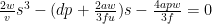
  north-south and


